Brave-Fox is a Firefox Theme that brings Brave’s design elements into Firefox.
Versions
There are two versions of Brave-Fox: Overflow & Non-Overflow.
Overflow vs Non-Overflow
Chromium-based browsers do this thing where with every new tab, each other tab gets smaller and smaller, till you open enough tabs that newer ones stop displaying after a certain number of tabs. Firefox said “nah”, and just decided to add a scroll wheel onto the tab bar.
Adding the Remove Overflow.css file to the Brave-Fox folder will disable Firefox’s tab scrolling and enable chromium-like tab behaviour.
Explanation
I highly recommend you read the documentation I spent hours on as it explains every line of code in each file, some also have before and after pictures to show off differences.
Installation
Install the pack you’d like to use, (including the Non-Overflow version if you’d like) (other than ReadMe.md).
Move all files to Chrome Folder
Add the following code to your userChrome.css & userContent.css files:
/*--------------------------------------------- Brave Fox --------------------------------------------*/@importurl("Brave-Fox/Import.css");
/*----------------------------------------------------------------------------------------------------*/
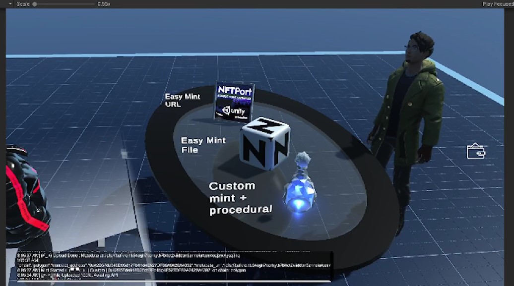
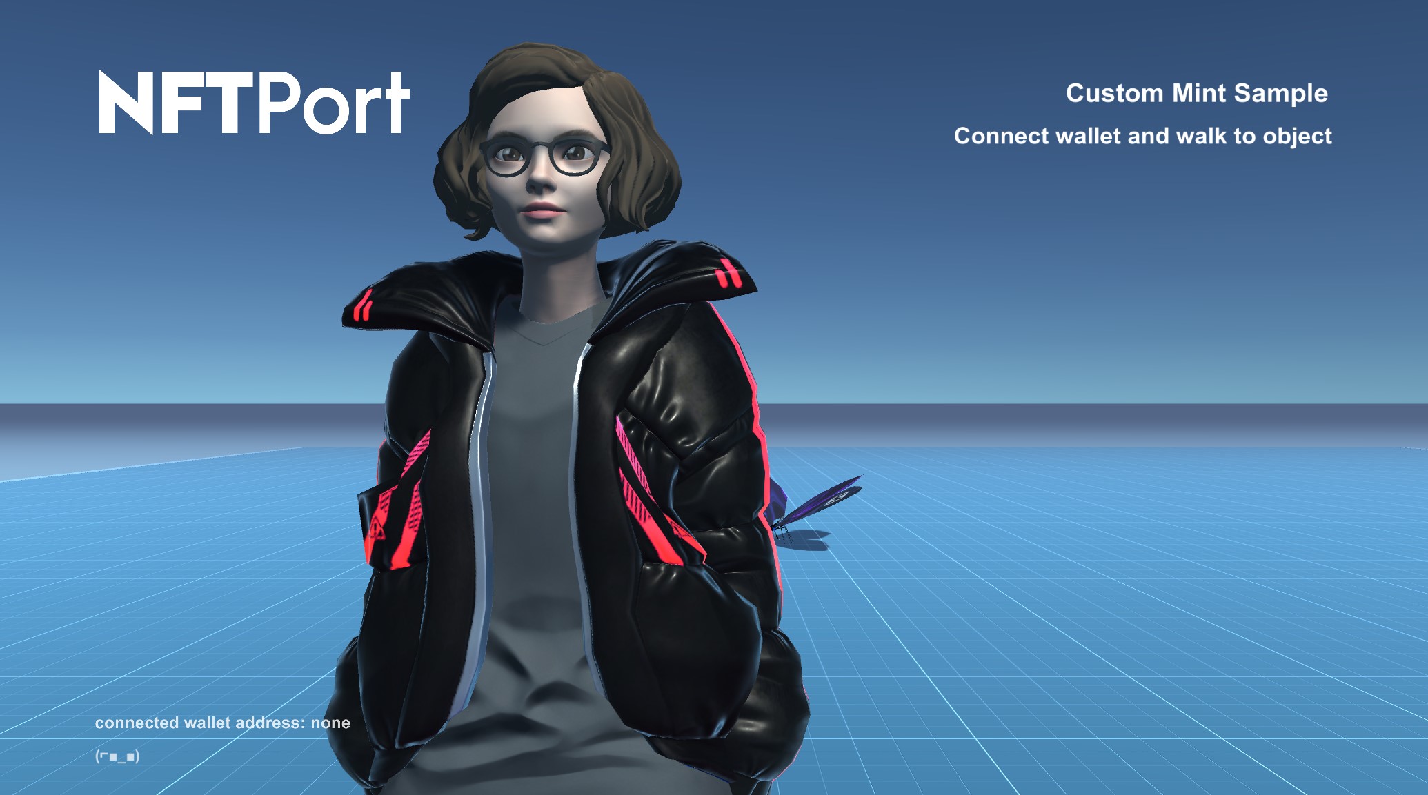
Advanced Playground showcases number of zones providing templates and demos for how to read/write-mint/update etc NFT data in game engine Unity.
Advanced Playground Mint zone:
Explore NFT minting shop template made in Unity3D to create cross-chain web3 games/metaverses including on Solana, Ethereum, polygon and more. In this showcase we generate a runtime custom NFT according to user input including procedural metadata, 3D object, NFT image and host it over IPFS, finally minting to our deployed collection to the connected players wallet.
A fully composable and ready to use gallery. Gallery Frames can be reduced or increased indefinately and put in any shape or formations according to your #metaverse needs.
A Phaser 3 project template with ES6 support via Babel 7 and Webpack 4 that includes hot-reloading for development and production-ready builds.
This has been updated for Phaser 3.50.0 version and above.
Loading images via JavaScript module import is also supported, although not recommended.
Requirements
Node.js is required to install dependencies and run scripts via npm.
Available Commands
Command
Description
npm install
Install project dependencies
npm start
Build project and open web server running project
npm run build
Builds code bundle with production settings (minification, uglification, etc..)
Writing Code
After cloning the repo, run npm install from your project directory. Then, you can start the local development server by running npm start.
After starting the development server with npm start, you can edit any files in the src folder and webpack will automatically recompile and reload your server (available at http://localhost:8080 by default).
Customizing the Template
Babel
You can write modern ES6+ JavaScript and Babel will transpile it to a version of JavaScript that you want your project to support. The targeted browsers are set in the .babelrc file and the default currently targets all browsers with total usage over “0.25%” but excludes IE11 and Opera Mini.
If you want to customize your build, such as adding a new webpack loader or plugin (i.e. for loading CSS or fonts), you can modify the webpack/base.js file for cross-project changes, or you can modify and/or create new configuration files and target them in specific npm tasks inside of `package.json’.
Deploying Code
After you run the npm run build command, your code will be built into a single bundle located at dist/bundle.min.js along with any other assets you project depended.
If you put the contents of the dist folder in a publicly-accessible location (say something like http://mycoolserver.com), you should be able to open http://mycoolserver.com/index.html and play your game.
Node module that synchronizes the files on a connected CircuitPython device to a local project folder. It provides a one-way sync from the CircuitPython device to the local project folder. Technically it does a copy rather than a sync, but if I included copy in the name, it would be cpcopy or cp-copy which looks like a merger of the Linux copy command cp plus the DOS copy command copy and that would be confusing.
When you work with a CircuitPython device, you generally read and write executable Python files directly from/to the device; there’s even a Python editor called Mu built just for this use case.
Many more experienced developers work with a local project folder then transfer the source code to a connected device, as you do when working with Arduino and other platforms. This module allows you to do both:
Read/write source code from/to a connected Circuit Python device using Mu or other editors (even Visual Studio Code plugins).
Automatically copy source files from the device to a local project folder whenever the change on the device.
Here’s how it works:
Create a local Python project with all the other files you need (like a readme.md file, or a .gitignore).
Connect a CircuitPython device to your computer.
Open a terminal window or command prompt and execute the module specifying the CircuitPython drive path and local project path as command line arguments.
The module copies all of the files from the connected CircuitPython device to the specified project folder.
Open any editor you want and edit the Python source code files (and any other file) on the connected device.
When you save any modified files on the connected CircuitPython device, the module automatically copies the modified file(s) to the project folder.
To install globally, open a command prompt or terminal window and execute the following command:
npm install -g cpsync
You’ll want to install globally since CircuitPython projects don’t generally use Node modules (like this one) so a package.json file and node_modules folder will look weird in your project folder.
Usage
To start the sync process, in a terminal window execute the following command:
<device_path> is the drive path for a connected CircuitPython device
<sync_path> is the local project folder where you want the module to copy the files from the connected CircuitPython device
Both command arguments are required (indicated by angle brackets < and >). Square brackets ([ and ])indicate optional parameters.
Options:
-d or --debug enables debug mode which writes additional information to the console as the module executes
-i or --ignore instructs the module to ignore the internal files typically found on a CircuitPython device.
A CircuitPython device hosts several internal use or housekeeping files that you don’t need copied into your local project. When you enable ignore mode (by passing the -i option on the command line), the module ignores the following when synchronizing files from the CircuitPython device to your local project folder:
If you find other device-side housekeeping files, let me know and I’ll update the ignore arrays in the module.
Examples
If you don’t want to install the module globally, you can execute the module on the fly instead using:
npx cpsync <device_path><sync_path>
On Windows, the device appears as a drive with a drive letter assignment. So, assuming it’s drive H (your experience may vary but that’s how it shows up on my Windows system) start the module with the following command:
cpsync h: c:\dev\mycoolproject
Assuming you’ll launch the module from your project folder, use a . for the current folder as shown in the following example:
cpsync h: .
On macOS, it mounts as a drive and you can access it via /Volumes folder. On my system, the device mounts as CIRCUITPY, so start the sync process using:
cpsync /Volumes/CIRCUITPY .
On Windows I like to execute the module from the terminal prompt in Visual Studio Code, but keep the terminal available to execute other commands, so I start the module using the following:
start cpsync <device_path><sync_path>
This starts the module in a new/separate terminal window, leaving the Visual Studio terminal available to me to execute additional commands.
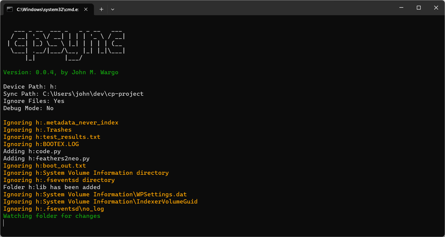
For example, if I execute the following command:
start cpsync h: . -i
A new window opens as shown in the following figure
The CircuitPython device shows up as drive H: and the . tells the module to copy the files to the current folder.
Every time you change the file contents on the device, the module copies the modified files to the local project folder.
Pull Requests gladly accepted, but only with complete documentation of what the change is, why you made it, and why you think its important to have in the module.
This is a Zotero plugin that allows you to rename PDF files in your Zotero library using custom rules.
Note: This plugin only works on Zotero 7.0 and above.
Usage
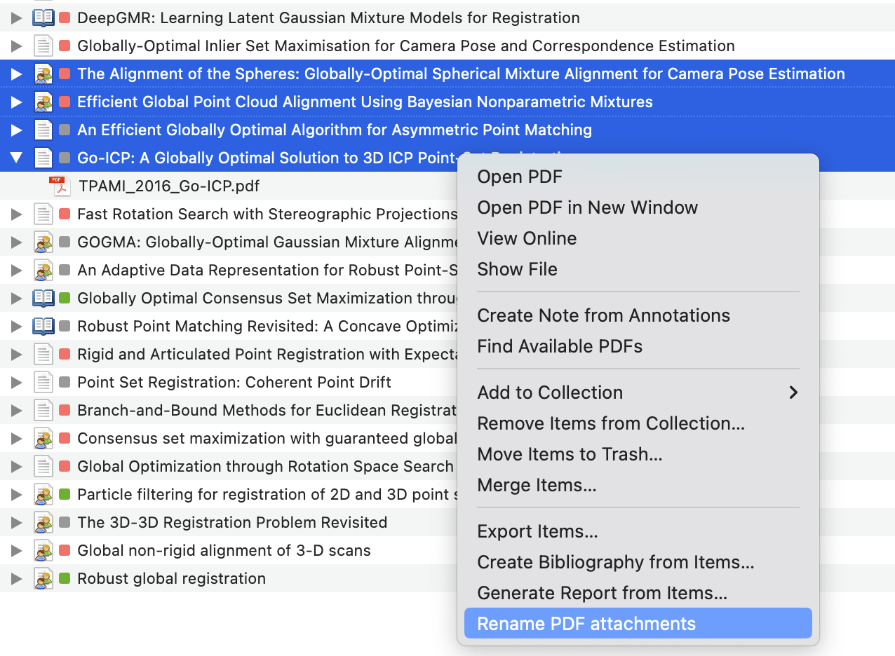
Select one or more items in your Zotero library and right click to open the context menu. Select Rename PDF attachments from the menu.
Then the PDF files will be renamed according to the custom rules you set in the plugin preferences(not implemented yet).
Default rules
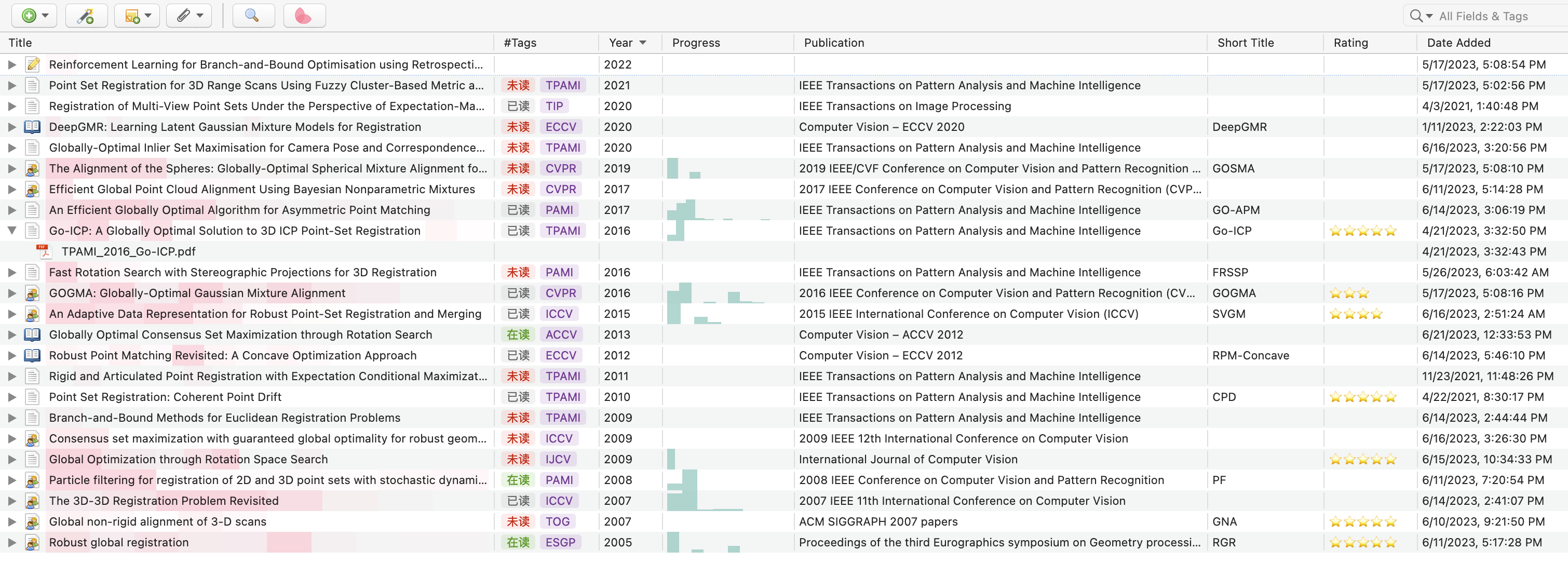
This plugin will read the journal name and year from the metadata of the item and rename the PDF file as follows:
{short journal name}_{year}_{short title}.pdf
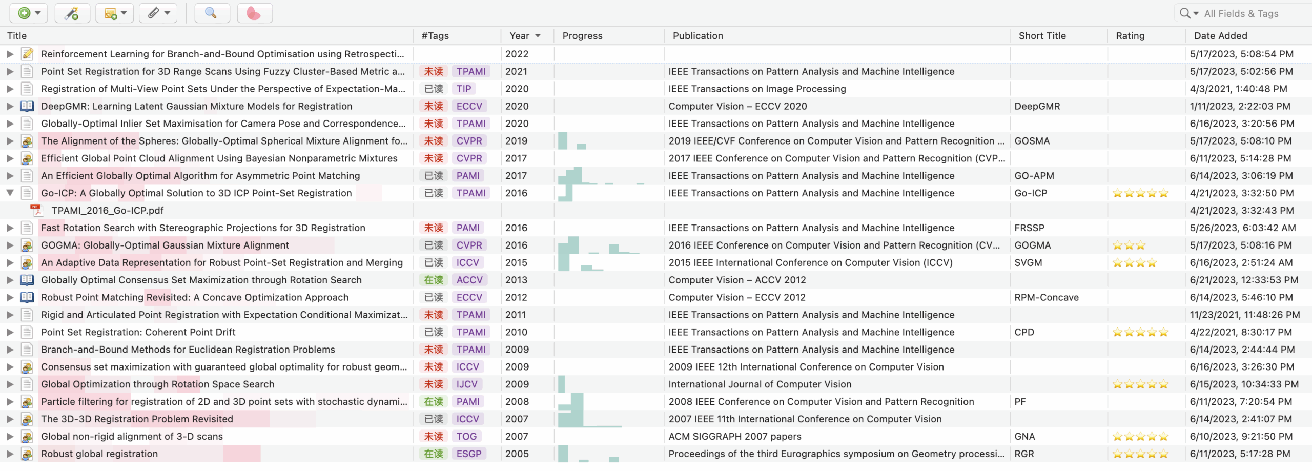
For example, the PDF file of the item below will be renamed as TPAMI_2016_Go-ICP.pdf.
The short title is read from the Short Title field of the item. If the Short Title field is empty, the plugin will use the Title field instead.
Journal tags
The short journal name is generated by selecting the first capital letter of each word in the journal name. For example, IEEE Transactions on Pattern Analysis and Machine Intelligence will be converted to TPAMI, while IEEE will be ignored.
However, ACM Transactions on Graphics will be converted to TG rather than TOG in current version. This is because the word on is ignored in the conversion.
A better method is manually adding the short name of the journal in the Tags of the item.
For example, you can add Jab/#TOG to the Tags of the item, and the plugin will use TOG as the short name of the journal.
Note: the plugin will first read the Jab/# tag in the Tags as the short name. If there is no Jab/# tag, the plugin will automatically extract the short name from the full name of the journal.
Now, we can use control+D to rename the PDF files. Moreover, we can customize the short cut in the Preferences of Zotero.
The custom short cut can be a combination of the modifier keys and another key. The modifier keys can be alt, control, meta and accel, while another key can be any key on the keyboard.
The following table shows the corresponding modifier keys on Windows and Mac.
modifier
Windows
Mac
alt
Alt
⌥ Option
control
Ctrl
⌃ Control
meta
❌ Not supported
⌘ Command
accel
Ctrl
⌘ Command
Future work
Add a short cut for the renaming function
Preferences panel to allow users to customize the rules.
Better way to extract the short name of the journal.
Tool, which generates graphql-go schema for .proto file.
Installation
$ go get github.com/saturn4er/proto2gql/cmd/proto2gql
Usage
To generate GraphQL fields by .proto
$ ./proto2gql
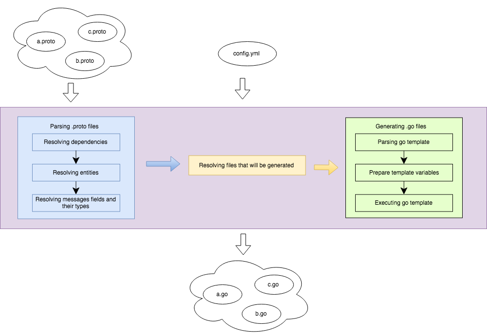
Generation process
Config example
paths: # path, where parser will search for imports
- "${GOPATH}/src/"generate_tracer: true # if true, generated code will trace all functions callsoutput_package: "graphql"# Common Golang package for generated files output_path: "./out"# Path, where generator will put generated filesimports: # .proto files imports settingsoutput_package: "imports"# Golang package name for generated importsoutput_path: "./out/imports"# Path, where generator will put generated imports filesaliases: # Global aliases for imports. google/protobuf/timestamp.proto: "github.com/gogo/protobuf/protobuf/google/protobuf/timestamp.proto"settings:
"${GOPATH}src/github.com/gogo/protobuf/protobuf/google/protobuf/timestamp.proto":
go_package: "github.com/gogo/protobuf/types"# golang package, of generated .proto filegql_enums_prefix: "TS"# prefix, which will be added to all generated GraphQL Enumsgql_messages_prefix: "TS"# prefix, which will be added to all generated GraphQL Messages(including maps)protos:
- proto_path: "./example/example.proto"# path to .proto file output_path: "./schema/example"# path, where generator will put generated fileoutput_package: "example"# Golang package for generated filepaths: # path, where parser will search for imports.
- "${GOPATH}/src/github.com/saturn4er/proto2gql/example/"gql_messages_prefix: "Example"# prefix, which will be added to all generated GraphQL Messages(including maps)gql_enums_prefix: "Example"# prefix, which will be added to all generated GraphQL Enumsimports_aliases: # imports aliasesgoogle/protobuf/timestamp.proto: "github.com/google/protobuf/google/protobuf/timestamp.proto"services:
ServiceExample:
alias: "NonServiceExample"# service name aliasmethods:
queryMethod:
alias: "newQueryMethod"# method name aliasrequest_type: "QUERY"# GraphQL query type (QUERY|MUTATION)messages:
MessageName:
error_field: "errors"# recognize this field as payload error. You can access it in interceptorsfields:
message_field: {context_key: "ctx_field_key"} # Resolver, will try to fetch this field from context instead of fetching it from argumentsschemas:
- name: "SomeSchema"# Schema nameoutput_path: "./out/schema.go"# Where generator will put fabric for this schemaoutput_package: "test_schema"# Go package name for schema filequeries:
type: "SERVICE"proto: "Example"service: "ServiceExample"filter_fields:
- "MsgsWithEpmty"exclude_fields:
- "excludedField"mutations:
type: "OBJECT"fields:
- field: "nested_example_mutation"type: "OBJECT"object_name: "NestedExampleMutation"fields:
- field: "ExampleService"type: "SERVICE"object_name: "ServiceExampleMutations"proto: "Example"service: "ServiceExample"filter_fields:
- "MsgsWithEpmty"
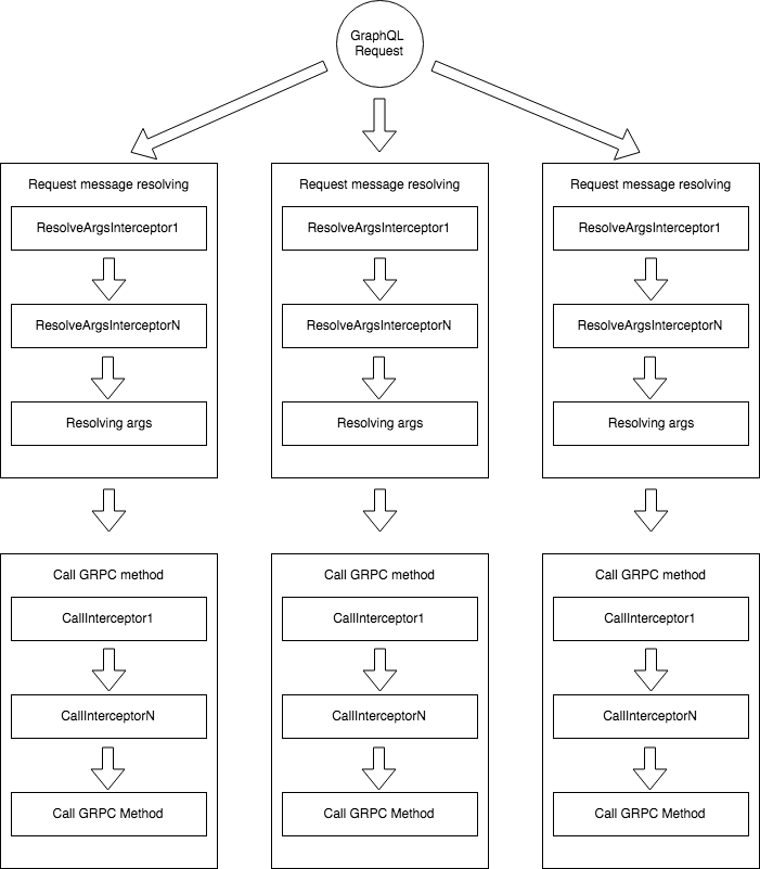
Interceptors
There’s two types of Interceptors. The first one can do some logic while parsing GraphQL arguments into request message and the second one, which intercept GRPC call. Here’s an example, how to work with it
Thanks for checking out this front-end coding challenge.
Frontend Mentor challenges help you improve your coding skills by building realistic projects.
To do this challenge, you need a basic understanding of HTML, CSS and JavaScript.
The challenge
Your challenge is to build out this dashboard and get it looking as close to the design as possible.
You can use any tools you like to help you complete the challenge. So if you’ve got something you’d like to practice, feel free to give it a go.
If you would like to practice working with JSON data, we provide a local data.json file for the activities. This means you’ll be able to pull the data from there instead of using the content in the .html file.
Your users should be able to:
View the optimal layout for the site depending on their device’s screen size
See hover states for all interactive elements on the page
Switch between viewing Daily, Weekly, and Monthly stats
Want some support on the challenge? Join our community and ask questions in the #help channel.
Expected behaviour
The text for the previous period’s time should change based on the active timeframe. For Daily, it should read “Yesterday” e.g “Yesterday – 2hrs”. For Weekly, it should read “Last Week” e.g. “Last Week – 32hrs”. For monthly, it should read “Last Month” e.g. “Last Month – 19hrs”.
Where to find everything
Your task is to build out the project to the designs inside the /design folder. You will find both a mobile and a desktop version of the design.
The designs are in JPG static format. Using JPGs will mean that you’ll need to use your best judgment for styles such as font-size, padding and margin.
If you would like the design files (we provide Sketch & Figma versions) to inspect the design in more detail, you can subscribe as a PRO member.
You will find all the required assets in the /images folder. The assets are already optimized.
There is also a style-guide.md file containing the information you’ll need, such as color palette and fonts.
Building your project
Feel free to use any workflow that you feel comfortable with. Below is a suggested process, but do not feel like you need to follow these steps:
Initialize your project as a public repository on GitHub. Creating a repo will make it easier to share your code with the community if you need help. If you’re not sure how to do this, have a read-through of this Try Git resource.
Configure your repository to publish your code to a web address. This will also be useful if you need some help during a challenge as you can share the URL for your project with your repo URL. There are a number of ways to do this, and we provide some recommendations below.
Look through the designs to start planning out how you’ll tackle the project. This step is crucial to help you think ahead for CSS classes to create reusable styles.
Before adding any styles, structure your content with HTML. Writing your HTML first can help focus your attention on creating well-structured content.
Write out the base styles for your project, including general content styles, such as font-family and font-size.
Start adding styles to the top of the page and work down. Only move on to the next section once you’re happy you’ve completed the area you’re working on.
Deploying your project
As mentioned above, there are many ways to host your project for free. Our recommended hosts are:
We strongly recommend overwriting this README.md with a custom one. We’ve provided a template inside the README-template.md file in this starter code.
The template provides a guide for what to add. A custom README will help you explain your project and reflect on your learnings. Please feel free to edit our template as much as you like.
Once you’ve added your information to the template, delete this file and rename the README-template.md file to README.md. That will make it show up as your repository’s README file.
Remember, if you’re looking for feedback on your solution, be sure to ask questions when submitting it. The more specific and detailed you are with your questions, the higher the chance you’ll get valuable feedback from the community.
Sharing your solution
There are multiple places you can share your solution:
Share your solution page in the #finished-projects channel of the community.
Tweet @frontendmentor and mention @frontendmentor, including the repo and live URLs in the tweet. We’d love to take a look at what you’ve built and help share it around.
Share your solution on other social channels like LinkedIn.
Blog about your experience building your project. Writing about your workflow, technical choices, and talking through your code is a brilliant way to reinforce what you’ve learned. Great platforms to write on are dev.to, Hashnode, and CodeNewbie.
We provide templates to help you share your solution once you’ve submitted it on the platform. Please do edit them and include specific questions when you’re looking for feedback.
The more specific you are with your questions the more likely it is that another member of the community will give you feedback.
Got feedback for us?
We love receiving feedback! We’re always looking to improve our challenges and our platform. So if you have anything you’d like to mention, please email hi[at]frontendmentor[dot]io.
This challenge is completely free. Please share it with anyone who will find it useful for practice.
Functional-Input Gaussian Processes with Applications to Inverse
Scattering Problems (Reproducibility)
Chih-Li Sung
December 1, 2022
This instruction aims to reproduce the results in the paper
“Functional-Input Gaussian Processes with Applications to Inverse
Scattering Problems” by Sung et al. (link). Hereafter, functional-Input
Gaussian Process is abbreviated by FIGP.
The following results are reproduced in this file
The sample path plots in Section S8 (Figures S1 and S2)
The prediction results in Section 4 (Table 1, Tables S1 and S2)
The plots and prediction results in Section 5 (Figures 2, S3 and S4
and Table 2)
Step 0.1: load functions and packages
library(randtoolbox)
library(R.matlab)
library(cubature)
library(plgp)
source("FIGP.R")                # FIGP
source("matern.kernel.R")       # matern kernel computation
source("FIGP.kernel.R")         # kernels for FIGP
source("loocv.R")               # LOOCV for FIGP
source("KL.expan.R")            # KL expansion for comparison
source("GP.R")                  # conventional GP
Step 0.2: setting
set.seed(1) #set a random seed for reproducingeps<- sqrt(.Machine$double.eps) #small nugget for numeric stability
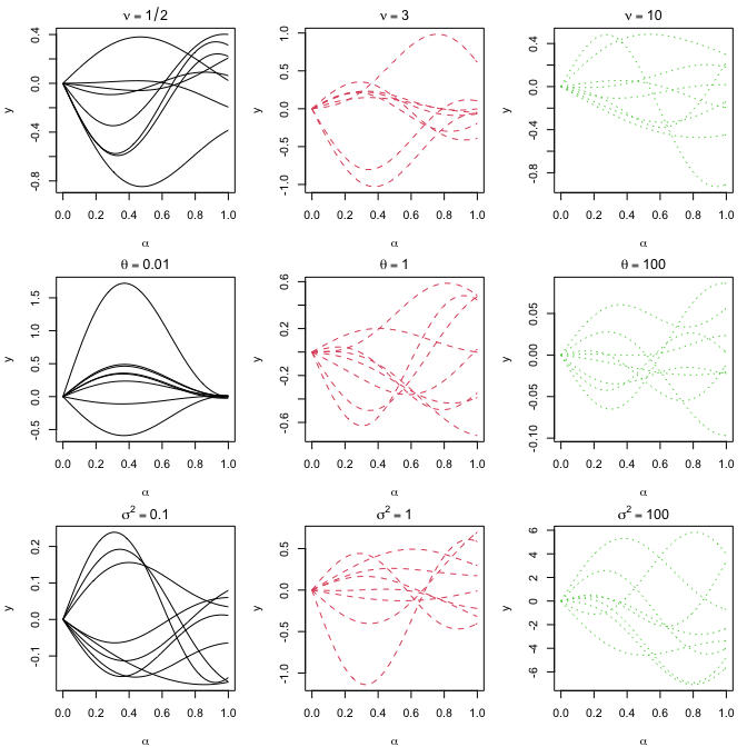
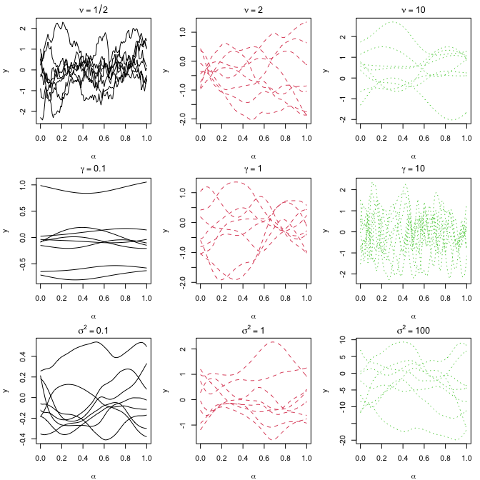
Reproducing Section S8: Sample Path
Set up the kernel functions introduced in Section 3. kernel.linear is
the linear kernel in Section 3.1, while kernel.nonlinear is the
non-linear kernel in Section 3.2.
with random $\alpha_1,\alpha_2, \beta$ and $\kappa$ from $[0,1]$.
# training functional inputs (G)G<-list(function(x) x[1]+x[2],
function(x) x[1]^2,
function(x) x[2]^2,
function(x) 1+x[1],
function(x) 1+x[2],
function(x) 1+x[1]*x[2],
function(x) sin(x[1]),
function(x) cos(x[1]+x[2]))
n<- length(G)
# y1: integrate g function from 0 to 1y1<- rep(0, n)
for(iin1:n) y1[i] <- hcubature(G[[i]], lower=c(0, 0),upper=c(1,1))$integral# y2: integrate g^3 function from 0 to 1G.cubic<-list(function(x) (x[1]+x[2])^3,
function(x) (x[1]^2)^3,
function(x) (x[2]^2)^3,
function(x) (1+x[1])^3,
function(x) (1+x[2])^3,
function(x) (1+x[1]*x[2])^3,
function(x) (sin(x[1]))^3,
function(x) (cos(x[1]+x[2]))^3)
y2<- rep(0, n)
for(iin1:n) y2[i] <- hcubature(G.cubic[[i]], lower=c(0, 0),upper=c(1,1))$integral# y3: integrate sin(g^2) function from 0 to 1G.sin<-list(function(x) sin((x[1]+x[2])^2),
function(x) sin((x[1]^2)^2),
function(x) sin((x[2]^2)^2),
function(x) sin((1+x[1])^2),
function(x) sin((1+x[2])^2),
function(x) sin((1+x[1]*x[2])^2),
function(x) sin((sin(x[1]))^2),
function(x) sin((cos(x[1]+x[2]))^2))
y3<- rep(0, n)
for(iin1:n) y3[i] <- hcubature(G.sin[[i]], lower=c(0, 0),upper=c(1,1))$integral
Reproducing Table S1
Y<- cbind(y1,y2,y3)
knitr::kable(round(t(Y),2))
y1
1.00
0.33
0.33
1.50
1.50
1.25
0.46
0.50
y2
1.50
0.14
0.14
3.75
3.75
2.15
0.18
0.26
y3
0.62
0.19
0.19
0.49
0.49
0.84
0.26
0.33
Now we are ready to fit a FIGP model. In each for loop, we fit a FIGP
for each of y1, y2 and y3. In each for loop, we also compute LOOCV
errors by loocv function.
loocv.l<-loocv.nl<- rep(0,3)
gp.fit<-gpnl.fit<- vector("list", 3)
set.seed(1)
for(iin1:3){
# fit FIGP with a linear kernelgp.fit[[i]] <- FIGP(G, d=2, Y[,i], nu=2.5, nug=eps, kernel="linear")
loocv.l[i] <- loocv(gp.fit[[i]])
# fit FIGP with a nonlinear kernelgpnl.fit[[i]] <- FIGP(G, d=2, Y[,i], nu=2.5, nug=eps, kernel="nonlinear")
loocv.nl[i] <- loocv(gpnl.fit[[i]])
}
As a comparison, we consider two basis expansion approaches. The first
method is KL expansion.
# for comparison: basis expansion approach# KL expansion that explains 99% of the variance
set.seed(1)
KL.out<- KL.expan(d=2, G, fraction=0.99, rnd=1e3)
B<-KL.out$BKL.fit<- vector("list", 3)
# fit a conventional GP on the scoresfor(iin1:3) KL.fit[[i]] <- sepGP(B, Y[,i], nu=2.5, nug=eps)
The second method is Taylor expansion with degree 3.
# for comparison: basis expansion approach# Taylor expansion coefficients for each functional inputtaylor.coef<-matrix(c(0,1,1,rep(0,7),
rep(0,4),1,rep(0,5),
rep(0,5),1,rep(0,4),
rep(1,2),rep(0,8),
1,0,1,rep(0,7),
1,0,0,1,rep(0,6),
0,1,rep(0,6),-1/6,0,
1,0,0,-1,-1/2,-1/2,rep(0,4)),ncol=10,byrow=TRUE)
TE.fit<- vector("list", 3)
# fit a conventional GP on the coefficientsfor(iin1:3) TE.fit[[i]] <- sepGP(taylor.coef, Y[,i], nu=2.5, nug=eps, scale.fg=FALSE, iso.fg=TRUE)
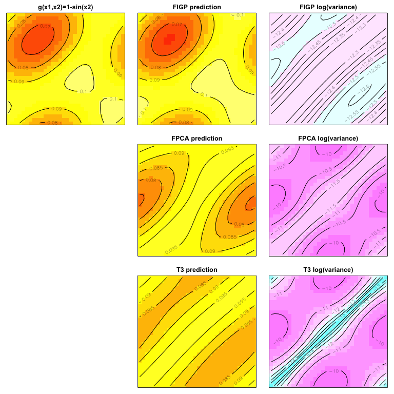
Let’s make predictions on the test functional inputs. We test n.test
times.
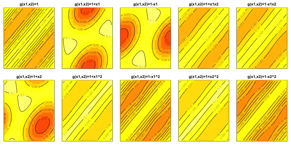
Now we move to a real problem: inverse scattering problem. First, since
the data were generated through Matlab, we use the function readMat in
the package R.matlab to read the data. There were ten training data
points, where the functional inputs are
$g(x_1,x_2)=1$
$g(x_1,x_2)=1+x_1$
$g(x_1,x_2)=1-x_1$
$g(x_1,x_2)=1+x_1x_2$
$g(x_1,x_2)=1-x_1x_2$
$g(x_1,x_2)=1+x_2$
$g(x_1,x_2)=1+x_1^2$
$g(x_1,x_2)=1-x_1^2$
$g(x_1,x_2)=1+x_2^2$
$g(x_1,x_2)=1-x_2^2$
Reproducing Figure 2
The outputs are displayed as follows, which reproduces Figure 2.
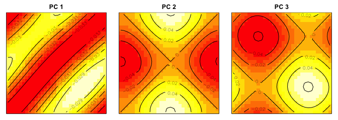
We perform PCA (principal component analysis) for dimension reduction,
which shows that only three components can explain more than 99.99%
variation of the data.
Foopipes generates markdown from the content found in Contentful CMS.
You can easily change how the markdown is generated for different content types by modifying the Typescript file ./modules_src/hugo.ts.
No need to rebuild or compile, just restart the Foopipes Docker container. (ctrl-c then docker-compose up)
How does it work?
Foopipes uses the configuration in foopipes.yml to fetch and process the content from Contentful.
It then invokes the Node module hugo to convert it markdown and then stores it to disk. Images (assets) are downloaded.
Hugo watches for changes and generates html files from the markdown.
Contentful webhooks
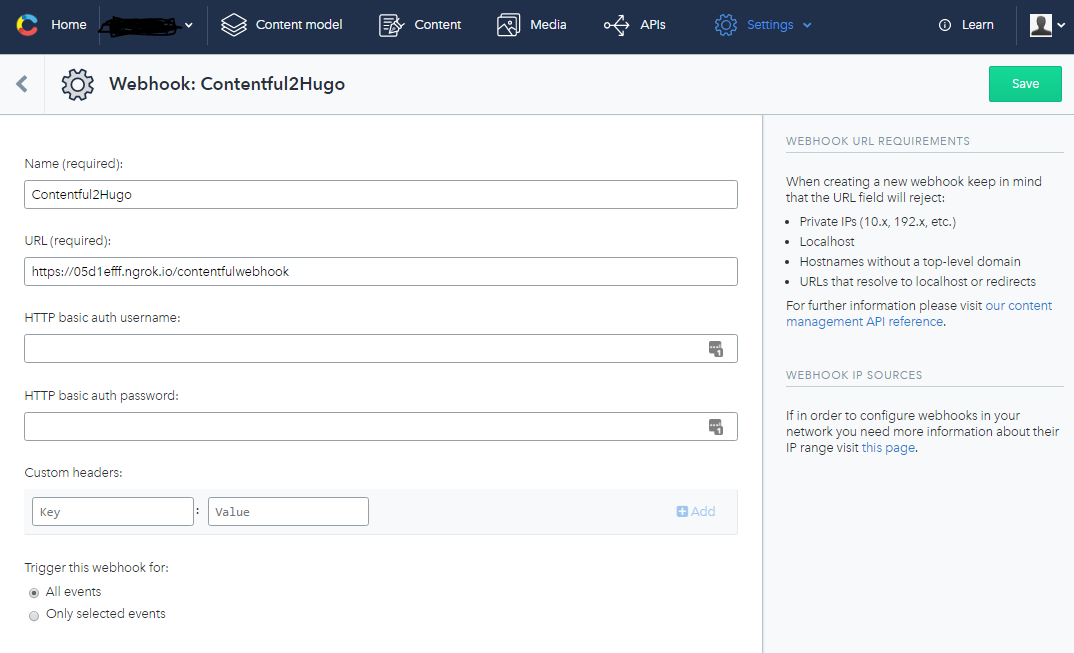
To avoid delays when editing in Contentful you can use Webhooks for immediate publish of changes.
In Contentful, configure a webhook endpoint to /contentfulwebhook in the Foopipes container port 80. (see below)
Contentful webhooks using ngrok
A helpful tool to allow incoming trafic through firewalls etc is https://ngrok.com/ which can be run inside a Docker container.
A Docker Compose configuration file is ready for use in this repository. It configured to run Hugo, Foopipes, ngrok and a nginx webserver.
Just start it with
Powershell:
$env:spaceId="<contentful_space_id>"
$env:accessToken="<contentful_acessToken>"
docker-compose up
Bash:
export spaceId=<contentful_space_id>
export accessToken=<contentful_acessToken>
docker-compose up
Important note about security
The webhook endpoint is not access restricted and open for anyone. If you exposed it to the internet, either directly or via ngrok, you must
consider the security issues that araises. It is recommended that you use some kind of proxy in front of the exposed endpoint to
limit access.


 https://github.com/Soft-Bred/Brave-Fox